Language Models From Scratch
Table of Contents
Background

Large Language models (LLMs) have marked an inflection point in software engineering and technology. I’ve been intrigued about the LLM architecture for some time now and so I decided to explore the foundational concepts behind the architecture from first-principles.
I approached this by reading the “Attention Is All You Need” paper — which introduced the Transformer architecture primarily used for LLMs today — while implementing the model from scratch in PyTorch.
After implementing the model architecture, I trained the model on a Machine Translation task of Igbo-English translations and the model achieved a BLEU score of 35.0 on a test dataset.
This post documents my observations and learnings from the project.
Language
Zooming in on the subject being modeled — we can describe language as an encoding system which allows us to describe, communicate and share information, ideas and abstract concepts in a format understood by a group of people.
Fundamentally, it is a social tool whose use spans multiple modalities, such as speech, text and sign language, given that an agreed set of symbols and words are established and understood by all parties who are involved in the use of the language.
A given language will contain a set of symbols, which serve as the atomic building blocks for constructing valid words. These words can then be assembled to communicate larger concepts.
Words can be combined together based on a syntax and set of grammatical rules which define the requirements for valid (coherent) sentences, which can be understood by users of the language.
The total set of words that can be used in a language form the vocabulary of the language.
Language = Tool for communication and information encoding.
Modeling/Model = To create a representative/imitated view of an underlying artifact/object/thing.
Machine Translation = Mapping a sequence of tokens from a given vector space \(V_a\) (the source language) to a sequence of tokens in another vector space \(V_b\)(the target language).
Implementation
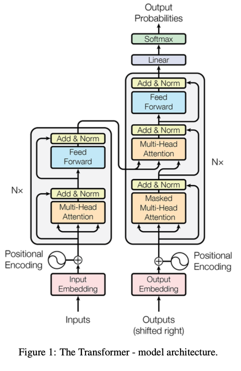
Based on the “Attention Is All You Need” paper":
There are several components of the architecture which we’ll need to build and I’ll be discussing the components that I found most interesting to implement:
- Tokeniser: Transforms a sentence containing words into tokens that are recognized in a given vocabulary.
- Vocabulary: Contains the total list of known tokens in a given language. Each token in the language’s vocabulary has a unique integer index which identifies it.
- Embedding layer: The embedding layer returns a learned embedding vector representing a given token, based on the token’s vocabulary index number.
- These vector representations of the token (embeddings) are learned over the course of training the model and eventually result in a learned latent space representing the vocabulary of words in the observed language.
- Positional Encoding: This returns an enriched vector embedding of the token, which includes information about the token’s position within the sequence.
- The token’s initial embedding is gotten from its vector representation in the vocabulary’s learned latent space, through the embedding layer. While that provides a valid vector representation of the token in isolation, it’s less helpful for our purposes, as this vector embedding doesn’t contain (spatial) context about the token’s order within a given sequence.
- Attention
- Multi-head Attention
- Cross-attention
- Masked Multi-head Attention
- Linear layer and Softmax: Generates the output probabilities based on the decoder’s output.
Tokeniser
In order to provide the model with features which describe the data, we need to transform our input and output sequence into tokens. These tokens will then be used to get the embedding vectors (i.e features) of the data.
A token’s embedding vector captures the semantic meaning of the token, and it is learned over the course of training the model.
A sequence could be a sentence in a given language (e.g English) or a single time-series sequence (e.g a stock ticker price at a point in time). For the sake of this task, our given sequence will be a sentence.
For a sentence in a given language, consisting of contiguous words and symbols, we want to compute its representation as a list of tokens.
A token is the smallest unit within the language’s vocabulary \(V\), this includes words, subwords and characters.
Each token \(T\) has a unique position \(V_T\) in the language’s vocabulary \(V\). This unique position is an integer, which is effectively the token’s index in the list of all tokens within the language.
A given language will be made up of a number of known tokens \(V_n\) which constitute its vocabulary \(V\)
I explored the following tokenisation strategies:
White-space Tokeniser
As a first-pass approach, I implemented a white-space tokeniser to transform a sentence into a list of tokens. This tokenizer naively splits a given sentence by white-space and special characters.
For example, a given sentence “Have a great day” gets encoded as ["Have", "a", "great", "day"].
This is simple to reason about — i.e a sentence can be tokenised as a list of words — and provides us with a quick tokenisation strategy which we can integrate with our model, right? Well, I quickly observed that this tokenisation strategy resulted in the number of parameters in the model exponentially increasing with the size of the dataset, which ultimately hurts model performance.
Why? A larger dataset will contain more sentences, which will contain more words. White-space tokenization takes a naive approach of considering each word before/after a white space as a token.
This comes with the cost of adding extra tokens to the vocabulary, due to new words being observed, which in turn increases the size of the embedding layer (vocabulary size x embedding dimension)
A better approach would be subword tokenization, such as Byte-Pair Encoding, where we can specify the size of the vocabulary i.e the number of unique tokens in the model’s latent space.
An added benefit of subword tokenization is that we can bound the vocabulary size and effectively handle out of distribution tokens by combining subwords.
Byte-Pair Encoding Tokeniser
Byte-pair Encoding (BPE) Tokenisation is a subword tokenisation algorithm that uses corpus statistics to determine how to encode a given sequence. The algorithm learns merge rules over a corpus based on the most frequently occurring pair of tokens i.e bi-grams.
By learning these merge rules, the algorithm learns how to tokenise words into sub-words.
For example, if the word “sing” appears frequently in our corpus, the BPE tokeniser might learn to tokenise words which have “sing” as the prefix:
This tokenisation approach enables the model better capture and encode meaning from words which have common parts. In the case of tokenising Singing -> [Sing, ing], the tokenisation rules allows us separate the verb sing from the gerund ing, which is the present participle suffix of the verb Singing. This would allow the model’s embeddings for the word Singing to encode both the action being performed and the tense.
BPE allows us specify the maximum number of merge rules that the algorithm needs to learn, which translates to specifying a vocabulary size. This gives us much more control over the number of parameters used by the model in its embedding layer, as it can be bounded.
The implication of using a sub-word tokeniser such as the Byte-Pair Encoding Tokeniser, is that we will now output more tokens when encoding a given sequence than the Whitespace Tokeniser. This is because each word will be split into subword tokens based on the learned merge rules, rather than a word per token.
To illustrate below, with BPE tokenisation we would encode the previous sequence “Have a great day” with 6 tokens rather than 4 tokens with Whitespace tokenisation:
I implemented the 🐙 Byte-Pair Encoding Tokeniser in Python for use in the model. While this implementation works great, it doesn’t utilize concurrency or threads, so the latency when learning merge rules is really high.
I consciously skipped this implementation detail primarily because concurrency is not a first-class feature in Python, so it felt less ergonomic to reach it for it, as opposed to if I was implementing the tokeniser in Go for example, which has much better concurrency APIs and support.
The latency in learning merge rules becomes incredibly clear when processing a large corpus, as we observe that tokenisation speed worsens as the dataset increases which is undesirable.
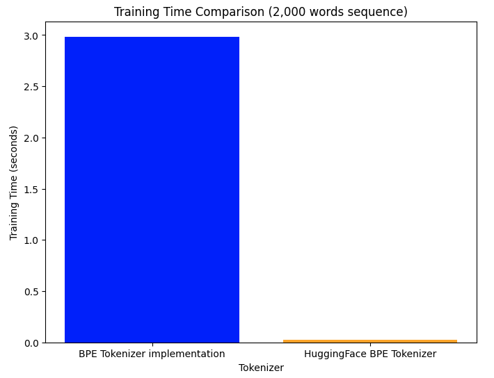

To workaround this latency constraint, I used the Hugging Face Tokenizers library (which is implemented in Rust, yay concurrency 🤠) to train a BPE tokeniser over the source and target sequences.
This resulted in a much shorter training time for the tokeniser; the training time and tokenisation speed are constant regardless of the size of the corpus.
Embeddings
The embeddings representing the semantic meaning of the tokens in a vector subspace across multiple dimensions.
We’ll have an embedding layer which will have \(V_n\) parameters, where \(V_n\) is the number of tokens in a given language’s vocabulary.
These embedding vectors are learnt over the course of training the model i.e the model learns how to best encode the meaning of a given token in its vector subspace based on the training criterion, which is accurate predictions in this case.
In other words, these vector representations will be modified as the model trains until it takes a form that allows the model to accurately predict the target sequence.
Positional encodings
Positional encodings allow the token embeddings to encode the position of each token within the sequence, improving the network’s understanding of how words relate to each other.
I like to think of positional encodings providing a way for tokens to encode spatial information within their token embeddings, which already contain semantic information about the token.
Each dimension in the word’s embedding has its positional encoding calculated as:
$$ \text{odd dimensions} = \sin\left(\frac{\text{pos}}{10{,}000^{\frac{2i}{\text{num_embeddings}}}}\right) $$
$$ \text{even dimensions} = \cos\left(\frac{\text{pos}}{10{,}000^{\frac{2i}{\text{num_embeddings}}}}\right) $$
We can plot the positional encoding value for 4-token long sequence “Have a great day” with 6 embedding dimensions:
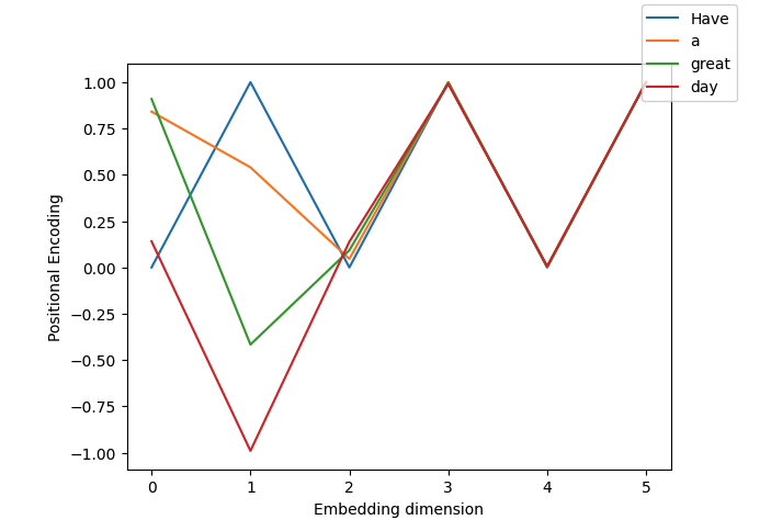
Taking the first token “Have” in the sentence as an example:
Before encoding, the token’s embeddings is:
[ 1.3686855, 2.4155787, 0.18680294, -1.5412053, -3.5412053, -0.5412053 ]
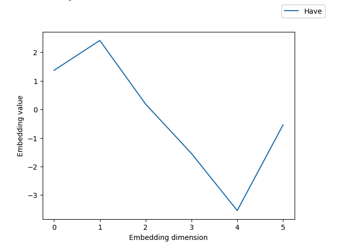
Given that it’s the first token in the sequence, its position pos = 0, so all odd dimensions will evaluate to sin(0) = 0.
All even dimensions will evaluate to cos(0) = 1.
This results in the below positional encoding vector for the token
[ 0.0, 1.0, 0.0, 1.0, 0.0, 1.0]
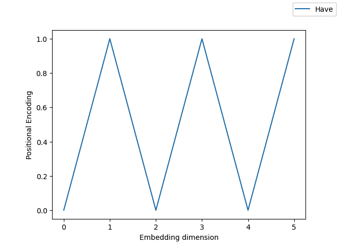
After adding the positional encoding with the token embedding, its embedding becomes:
[ 1.3687, 2.4156, 0.1868, -1.5412, -3.5412, -0.5412]
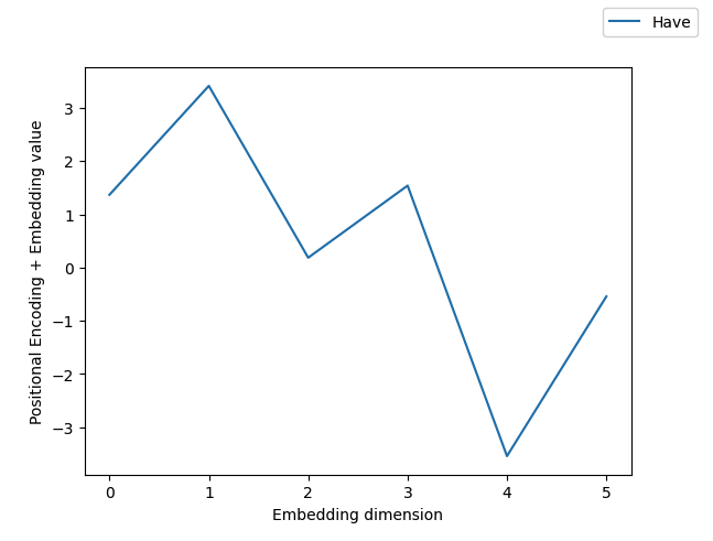
We can compare the updated token embeddings before and after positional encodings are applied:
Attention
Attention allows us pass information about a given token to other tokens in the sequence.
This allows the token get context on its usage within the sentence.
We can compute attention with the formula:
$$ Attention(Q, K, V) = softmax(\frac{QK^T}{\sqrt{d_k}})V $$
Where \(Q\), \(K\) and \(V\) are the query, key and value vectors respectively. \(\sqrt{dk}\) refers to the square root of the number of embedding dimensions in the key projection.
The dot product \((Q.K^T)\) of the query and keys results in a square-shaped (Context Length X Context Length) vector that outlines the raw attention scores for each word against every other word.
The \(\sqrt{dk}\) allows us scale the attention scores relative to the embedding dimensions being used in the model for the keys projection. The softmax operation normalizes the attention scores, ensuring that the sum of the attention scores for a given token is 1.
Finally, the scaled attention score is multiplied with the values \(V\) to get an embedding result for token, which will contain attention/context from other tokens.
Attention Linear Projections
Given the source sequence “nnukwu ụbọchị” in igbo — which translates to “great day” — with 6 embedding dimensions for each token:
| Token | Embedding |
|---|---|
| nnukwu | [-1.3, 3.1, 7.3, 2.54, -2.54, -0.54] |
| ụbọchị | [-2.4, 4.1, 8.3, 1.54, -3.54, -0.54] |
In order to get the queries, keys and values to use for attention we perform 3 linear transformations on the embeddings using learned weights: \(W_Q\), \(W_K\) and \(W_V\).
Taking a single token “ụbọchị” as an example, its attention linear projection in the encoder would look like:
We will perform the same linear projection for the token “nnukwu” and then we’ll calculate attention using the embeddings from the linear projections:
$$ Attention(Q, K, V) = softmax(\frac{QK^T}{\sqrt{d_k}})V $$
$$ \text{where } Q = Q_iW_Q, K = K_iW_K, V = V_iW_V $$
$$ \text{where } Q_i = K_i = V_i = \text{Embedding for token i} $$
The choice of what embedding value to use for the attention calculation/projections will vary based on the type of attention which is being performed.
In the case of self-attention, the query, key and value embeddings are all the same i.e either the encoder or decoder embeddings.
In the case of cross-attention, the query embeddings are the decoder embeddings, while the key and value embeddings are the encoder embeddings.
Attention Types
We perform 3 types of attention in the model:
- Encoder Self-attention: Allows the source sequence to attend to itself.
- Decoder Self-attention: Allows the target sequence to attend to itself.
- Encoder-Decoder Attention / Cross-attention: Allows every position in the target sequence to attend to all positions in the source sequence.
Multi-head attention
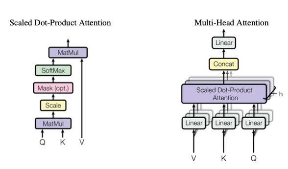
We perform the attention computation \(h\) times, where \(h\) is the number of attention heads. By using multiple attention heads, the model can jointly attend to information from different representation subspaces at different positions.
This also means that we’ll perform the queries, keys and values linear projection \(h\) times.
Finally, we concatenate the results of the attention heads and pass them through a linear layer to get the final multi-head attention output.
I like to think of each attention head as a domain-specialist within the model, which focuses on a range of semantic topics. By assembling multiple of these attention heads, the model learns various semantic structures across various vector subspaces.
Attention terminology
The attention definition borrows some terms from information retrieval systems such as databases, where we query (search) for a given value (e.g a user), which is stored by a given key (e.g user id). In this case, we want to query for how much attention a word should pay to every other word in the sequence.
Understanding the origin of the terms still didn’t help understand why exactly these 3 transformations are needed, why not 4 linear transformations?
The intuition here is that during training the model learns to:
- Set its weights used for each linear projection in a way that captures the token’s meaning in a subspace.
- Compute attention score logits \(Q.K^T\) that scale the values transformation \(V\) in a way that leads to accurate predictions.
Visualising Attention
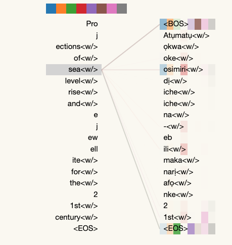
We can visualise how each word in a source sequence attends to every other word in a target sequence with the following interactive example below, which allows to view the attention weights for each layer.
The below example is interactive. Each square colored block represents an attention head in the selected layer. The attention head blocks can be double clicked to view the specific attention weights for the head.
| Sequence Type | Sequence Value |
|---|---|
| Source Sentence (Igbo) | Atụmatụ ọkwa oke osimiri dị iche iche na - ebili maka narị afọ nke 21st |
| Target Sentence (English) | Different sea level rise projections for the 21st century |
| Predicted Sentence | Projections of sea level rise and ejewellite for the 21st century |
For reference, Google translate predicts the following:
| Sequence Type | Sequence Value |
|---|---|
| Source Sentence (Igbo) | Atụmatụ ọkwa oke osimiri dị iche iche na - ebili maka narị afọ nke 21st |
| Target Sentence (English) | Different sea level rise projections for the 21st century |
| Google Translate Output Sentence (English) | Different ocean plans are rising for the 21st century |
While the model doesn’t accurately predict the english translation and it inserts an incorrect word ejewellite 😂, it’s able to capture the overall meaning of the words in the source sentence and translate them to the target sentence.
⭐️ Interpreting Attention Weights
In the interactive example above which visualizes the attention weights, I found that the last layer of the model were usually the most interpretable, as it contains the accumulated context of the previous layers.
The cross-attention weights in the last layer are also interesting, as they provide a view of how the source sequence attends to the target sequence.
For example, in the the last layer’s cross attention weights, we can see that the English word ‘sea’ in the predicted sentence pays the most attention to the Igbo word ‘osimiri’ which means ‘river’ in English.
Causal Masking
When training the model, we use a training technique called “Teacher Forcing” which involves providing the model with the complete target sequence during training but masking the future tokens in any given position.
We don’t want the model to predict the next token based on the position of future tokens, as that would defeat the purpose of the model’s learning task.
We want the predictions to be causal i.e if this then that. This allows us frame the learning task as thus — “given previously observed information, what comes next?”.
This need for masking becomes relevant in the model’s decoder self-attention layer during training which applies attention on the full target sequence.
In order to achieve causal masking, we generate a mask tensor, which is effectively a square shaped (context_length x context_length) tensor. Each row in the tensor corresponds to a word and each column indicates whether that word should attend to a neighboring word in that position.
This mask tensor is applied to the computed attention scores before the softmax operation, ensuring that the resulting attention weights respect the causal constraint. The mask is applied by adding a large negative value (e.g., negative infinity−∞) to the attention scores corresponding to future positions.
The softmax function converts the adjusted attention scores into probabilities. By masking these future positions (i.e setting them to large negative values) ahead of the softmax operation, we effectively get back zero probabilities for these positions. This ensures that future positions do not influence the model’s prediction for a given position.
For example, given a target sequence of tokens [x1, x2, x3, x4] during training, when predicting x3, the model should only attend to x1 and x2 but not x4.
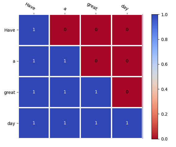
In the above diagram, blue box columns (1 values) indicate tokens which should be attended to.
The red box columns (0 values) indicate tokens which should not be attended to by the current word (token) on that row. These are the future words for that position.
As highlighted, only previous words can be attended to in order to predict the next word.
Linear layer and Softmax
The model’s outputs are gotten from the linear layer followed by a softmax over the raw logits.
The linear layer is a simple 1-layer block which takes in a (batch size, context length, embedding dimension) shaped tensor and outputs a (batch size, context length, vocabulary size) shaped tensor.
💡 Intuitively, this means that the layer takes in the embeddings for each token in a given input sequence within a batch. The embeddings for each token are used as inputs to map to target tokens in the target sequence’s vocabulary. Each token will have \(N\) possible outputs, where \(N\) is the vocabulary size.
This transformation/mapping which is performed by the linear layer allows the model to map the accumulated context (memory) from the source sequence and the available target sequence to the target sequence’s vocabulary vector space, which will contain \(N\) potential words (where \(N\) is the vocabulary size)
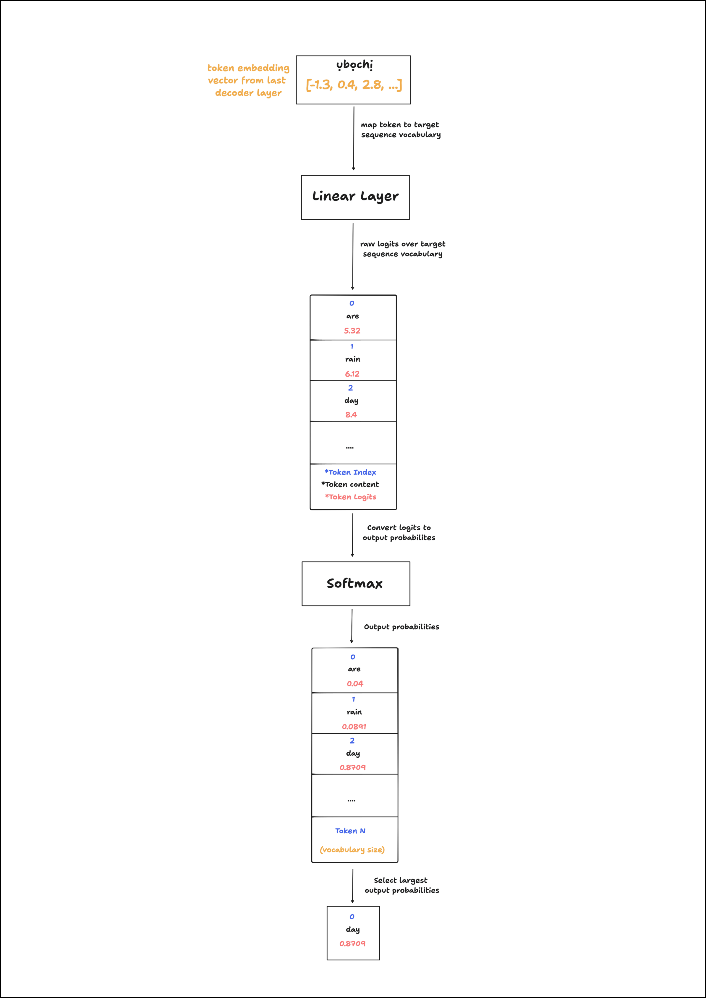
This projection from accumulated context (memory) to the target sequence’s vocabulary space allows the model to predict the next word for a given position (given an appropriate target and loss function of course).
Finally, we perform a softmax operation on the outputs of the linear layer, which we refer to as the logits. The softmax operation returns output probabilities where the sum of all the probabilities equals 1. This allows us better represent how confident a model’s prediction for a given potential target token is.
Training
The Wikimedia Dataset was used for training which contains 174,918 English-Igbo sentence pairs.
In future iterations, I would like to run evals on the Masakhane English-Igbo Machine Transalation eval dataset and The JW300 English-Igbo dataset.
This 🔗 dataset also looks promising.
Scheduler
When training the model I utilized a scheduled learning rate using the formula suggested in paper:
$$ \text{lrate} = d_{\text{model}}^{-0.5} \cdot \min(\text{step_num}^{-0.5}, \text{step_num} \cdot \text{warmup_steps}^{-1.5}) $$
The above formula increases the learning rate (from 0) for the first N warmup steps, after which the learning rate is gradually decreased.
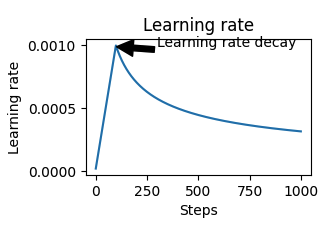
The computed learning rate is relative to the number of embedding dimensions used by model.
I observed much better results and less overfitting when training with the scheduled learning rate rather than a fixed learning rate.
Results
| Metric | Value |
|---|---|
| Training Loss | 2.1 |
| Eval Loss | 2.7 |
| Eval BLEU score | 48.3 |
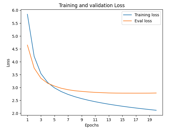
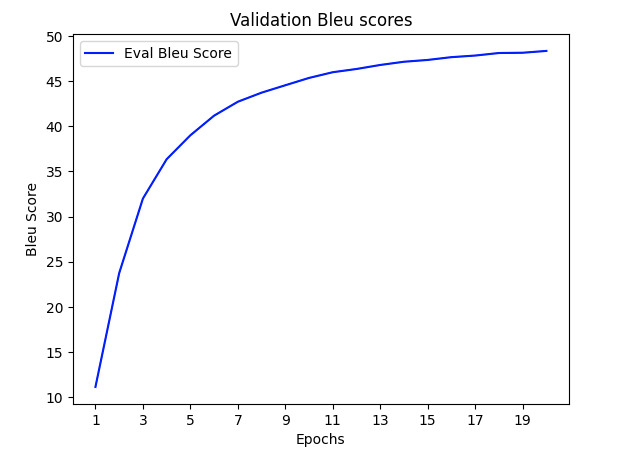
The model was trained for 20 epochs on a dataset of 170,000 English-Igbo sentence pairs with the following hyper-parameters:
| Hyper-Parameter | Value |
|---|---|
| Embedding Dimensions | 512 |
| Attention Heads | 8 |
| Context Length | 30 |
| FFN Dimensions | 2048 |
| Number of Layers | 6 |
| Dropout Probability | 0.1 |
| Label Smoothing | 0.1 |
| Scheduled Learning Rate? | True |
| Warm-up Steps | 100 |
| Base Learning Rate | 0.15 |
Takeaways
Language modeling is a really interesting domain, it allows us peak into the underlying structure of a language, and extract useful and generalizable features.
I had loads of fun working on this and I’m excited to explore improvements to the Transformer architecture and other (natural) language modeling approaches such as mixture of experts, rotary embeddings and sparse autoencoders.
I’m also excited to explore reinforcement learning and its application in grounding language models in real word scenarios and expectations. Particularly looking forward to this, so I can finally put some of that first year Psychology knowledge to use :p (hopefully it’s extrapolatable).
Code
Github Repository: https://github.com/darthchudi/transformer-py
🕹️ Replicate Model Demo: https://replicate.com/darthchudi/igbo_to_english_llm


